Contents
%%Uso de formato largo: mejores soluciones
format long
Ejercicio 1
x = [10; 20; 40; 60; 80];
y = [x, log(x)];
fprintf('\n Numero Natural log\n')
fprintf('%4i \t %8.3f\n',y')
 Numero Natural log
  10 	    2.303
  20 	    2.996
  40 	    3.689
  60 	    4.094
  80 	    4.382
Ejercicio 2
A = [4 -2 -10; 2 10 -12; -4 -6 16];
b = [-10; 32; -16];
disp('Solucion')
x = inv(A)*b
disp('Comprobacion')
A*x - b %prueba
Solucion

x =

     2
     4
     1

Comprobacion

ans =

     0
     0
     0
Ejercicio 3
A = [4 -2 -10; 2 10 -12; -4 -6 16];
b = [-10; 32; -16];
disp('L U')
[L U] = lu(A)
disp('Solucion')
x = inv(U)*inv(L)*b
disp('Comprobacion')
A*x - b %prueba
L U

L =

   1.000000000000000                   0                   0
   0.500000000000000   1.000000000000000                   0
  -1.000000000000000  -0.727272727272727   1.000000000000000


U =

   4.000000000000000  -2.000000000000000 -10.000000000000000
                   0  11.000000000000000  -7.000000000000000
                   0                   0   0.909090909090909

Solucion

x =

     2
     4
     1

Comprobacion

ans =

     0
     0
     0
Ejercicio 4
A = [ 0 1 -1; -6 -11 6; -6 -11 5 ];
[x, D] = eig(A)
T1 = A*x
T2 = x*D
x =

   0.707106781186543  -0.218217890235999  -0.092057461789830
   0.000000000000004  -0.436435780471979  -0.552344770738996
   0.707106781186551  -0.872871560943971  -0.828517156108490


D =

  -1.000000000000005                   0                   0
                   0  -1.999999999999970                   0
                   0                   0  -3.000000000000024


T1 =

  -0.707106781186547   0.436435780471991   0.276172385369494
  -0.000000000000002   0.872871560943942   1.657034312217000
  -0.707106781186553   1.745743121887913   2.485551468325490


T2 =

  -0.707106781186547   0.436435780471991   0.276172385369494
  -0.000000000000004   0.872871560943945   1.657034312217002
  -0.707106781186555   1.745743121887915   2.485551468325490
Ejercicio 5
A = [(1.5 - 2i) (-0.35 + 1.2i); (-0.35 + 1.2i) (0.9 -1.6i)];
b = [(30 + 40i); (20 + 15i)];
v = inv(A)*b;
disp('Solución:')
V1 = v(1)
V2 = v(2)
S = v.*conj(b)
Solución:

V1 =

  3.590204703232966 +35.092792858473679i


V2 =

  6.015537032086641 +36.221212342138735i


S =

   1.0e+03 *

  1.511417855435936 + 0.909175597624892i
  0.663628925773814 + 0.634191191361475i
Ejercicio 6
Resuelve las torres de Hanoi function hanoi (n, i, a, f) if n > 0 hanoi (n - 1, i, f, a); fprintf('mover disco %d de %c a %c\n', n, i, f); hanoi (n - 1, a, i, f); end
hanoi(3, 'i', 'a', 'f')
mover disco 1 de i a f
mover disco 2 de i a a
mover disco 1 de f a a
mover disco 3 de i a f
mover disco 1 de a a i
mover disco 2 de a a f
mover disco 1 de i a f
Ejercicio 7
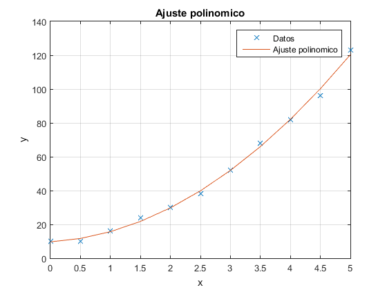
figure(7)
x = 0:0.5:5;
y = [10 10 16 24 30 38 52 68 82 96 123];
p = polyfit(x,y,2);
yc = polyval(p,x);
plot(x,y,'x',x,yc)
xlabel('x'),ylabel('y'),grid,title('Ajuste polinomico')
legend('Datos','Ajuste polinomico',4)
Ejercicio 8
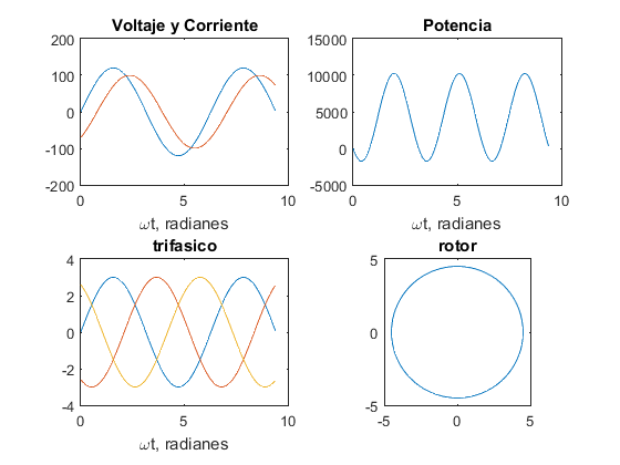
figure(8)
wt = 0:0.05:3*pi;
v = 120*sin(wt);
i = 100*sin(wt-pi/4);
p = v.*i;
subplot(2,2,1)
plot(wt,v,wt,i)
title('Voltaje y Corriente'),xlabel('\omegat, radianes')
subplot(2,2,2)
plot(wt,p)
title('Potencia'),xlabel('\omegat, radianes')
Fm = 3.0;
fa = Fm*sin(wt);
fb = Fm*sin(wt-2*pi/3);
fc = Fm*sin(wt-4*pi/3);
subplot(2,2,3)
plot(wt,fa,wt,fb,wt,fc)
title('trifasico'),xlabel('\omegat, radianes')
fR = 3/2*Fm;
subplot(2,2,4)
plot(-fR*cos(wt),fR*sin(wt))
title('rotor'),axis square
Ejercicio 9

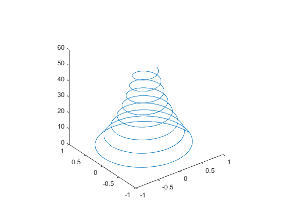
t = 0:0.1:16*pi;
x = exp(-0.03*t).*cos(t);
y = exp(-0.03*t).*sin(t);
z = t;
subplot(1,1,1)
plot3(x,y,z), axis square
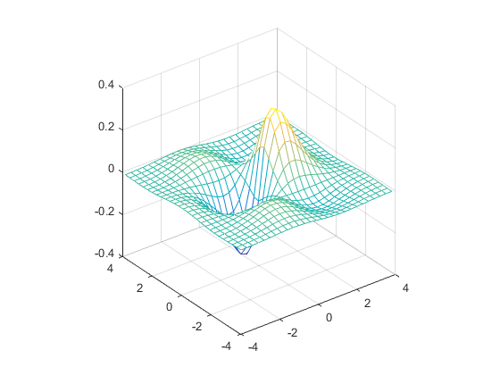
Ejercicio 10

t= -4:0.3:4;
[x,y]=meshgrid(t,t);
z=sin(x).*cos(y).*exp(-(x.^2+y.^2).^0.5);
mesh(x,y,z) , axis square
Ejercicio 11

q = [1 0 -35 50 24]; %Matriz de coeficientes del polinomio
disp('Raices')
r = roots(q) %Raices del polinomio
disp('Comprobacion')
polyval(q,r) %Evaluar valores del polinomio con las raices -> [0]
Raices

r =

  -6.491019200948975
   4.870585123318113
   2.000000000000000
  -0.379565922369139

Comprobacion

ans =

   1.0e-11 *

  -0.141398004416260
  -0.065014660322049
  -0.003552713678801
  -0.000355271367880
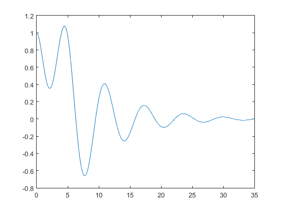
Ejercicio 12
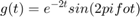
figure(12)
Ejemploode
% function Ejemploode
% [t, yy] = ode45(@HalfSine, [0 35], [1 0], [], 0.15);
% plot(t, yy(:,1))
% function y = HalfSine(t, y, z)
% h = sin(pi*t/5).*(t<=5);
% y = [y(2); -2*z*y(2)-y(1)+h];
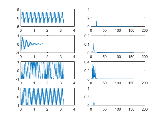
Ejercicio 13


figure(13)
k = 5;   m = 10;   fo = 10;   Bo = 2.5;
N = 2^m;   T = 2^k/fo;
ts = (0:N-1)*T/N;
df = (0:N/2-1)/T;
SampledSignal = Bo*sin(2*pi*fo*ts) + Bo/2*sin(2*pi*fo*2*ts);
An = abs(fft(SampledSignal, N))/N;
subplot(4,2,1)
plot(ts, SampledSignal)
subplot(4,2,2)
plot(df, 2*An(1:N/2))

SampledSignal1 = exp(-2*ts).*sin(2*pi*fo*ts);
An1 = abs(fft(SampledSignal1, N))/N;
subplot(4,2,3)
plot(ts, SampledSignal1)
subplot(4,2,4)
plot(df, 2*An1(1:N/2))

SampledSignal2 = sin(2*pi*fo*ts + 5*sin(2*pi*fo/10*ts));
An2 = abs(fft(SampledSignal2, N))/N;
subplot(4,2,5)
plot(ts, SampledSignal2)
subplot(4,2,6)
plot(df, 2*An2(1:N/2))

SampledSignal3 = sin(2*pi*fo*ts - 5*exp(-2*ts));
An3 = abs(fft(SampledSignal3, N))/N;
subplot(4,2,7)
plot(ts, SampledSignal3)
subplot(4,2,8)
plot(df, 2*An3(1:N/2))
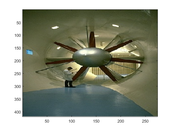
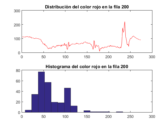
Ejercicio 14
figure(14)
A = imread('WindTunnel.jpg', 'jpeg');
image(A)
row = 200;
red = A(row, :, 1);
gr  = A(row, :, 2);
bl  = A(row, :, 3);
figure(141)
subplot(2,1,1)
plot(red, 'r');
title('Distribución del color rojo en la fila 200');
%hold on
%plot(gr, 'g');
%plot(bl, 'b');
subplot(2,1,2)
hist(red,0:15:255);
title('Histograma del color rojo en la fila 200');
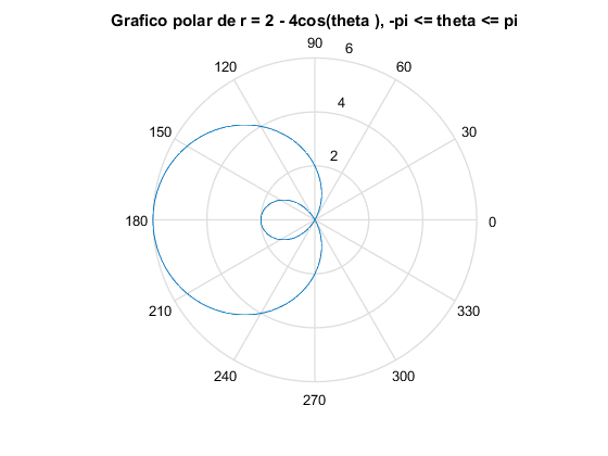
Ejercicio 15

theta = linspace(-pi, pi, 180);
r = 2 - 4*cos(theta);
figure(15)
polar(theta, r);
title('Grafico polar de r = 2 - 4cos(theta ), -pi <= theta <= pi');